4 six sided die, labeled a-d, with weights denoted by the following vectors
a -> equally weighted
b -> \(( 0.1,0.3,0.1,0.1,0.3,0.1 )\)
c -> \(( 0.1, 0.2, 0.1, 0.15, 0.25, 0.2 )\)
d -> \(( 0.15, 0.2, 0.05, 0.1, 0.2, 0.3 )\)
2 coins labeled 1 and 2 with the following probability p for heads
1 -> p = .75
2 -> p = .25
Instructions:
Shuffle the cards together to obtain a well mixed deck
Draw a card from the deck. Record the suit
For each suit:
If hearts, choose die a
If diamonds, choose die b
If spades, choose die c
If clubs, choose die d
Record which die you choose
If die a or c, grab coin 1
If die b or d, grab coin 2
Roll the die
Call the number on the face of the die N
Flip the coin you grabbed N times
Count the number of tails you get
Possible outcomes: \(0, 1, 2, 3, 4, 5, 6\)
Analysis
Let us solve this problem directly. Define the random variable \(X\) = # of tails flipped. We can now use LOTP to find \(P(X=k)\) conditioning on which die we roll. So this will look like
We know still that \(P(\textrm{a})=P(\textrm{b})=P(\textrm{c})=P(\textrm{d})=1/4\), as the die gets chosen by drawing a card from a shuffled deck of 52 cards, and looking at the suit with each suit equally likley. Let us now consider \(P(X=k|\textrm{a})\). In order to solve this for any of the terms in our LOTP we have here, we will again have to make use of the LOTP, this time conditioning on which number gets rolled on the die. So doing this we have,
\[
P(X=k|a)=\sum_{j=1}^6P(X=k|a,Rj)P(Rj|a).
\] Where \(Rj\) is the event of rolling the number \(j\) on the die. We can similarly write this for all of our conditional terms in our original LOTP.
Now note that in each case, the probability \(P(Rj|die)\) is given by the probability vectors of each respective die given at the beginning of the experiment. So we would like to calculate our probabilities \(P(X=k|a,Rj)\). Note that for any given die, we know which coin we have. For dies \(a\) and \(c\), we have coin one with probability \(p = .75\) of heads. For dies \(b\) and \(d\), we have coin two with probability \(p = .25\) of heads. So all the condition of which die we has does for our probability is tell us which coin we have. We are then just looking at \(P(X=k|Rj)\) which will be distributed \(Bin(1-p,j)\) for whatever \(p\) corresponds to the coin we are flipping. This is because we have a \(p\) coin, and we are flipping it \(j\) times, however we are counting the number of tails we get. So this is \(Bin(1-p,j)\). We can calculate all these probabilities for each coin and store them in a matrix.
So we now have two matrices denoting our probabilities \(P(X=k|\textrm{Rj})\) for coin 1, which corresponds to dices \(a\) and \(c\), and coin 2 which corresponds to dices \(b\) and \(d\). We can now use these matrices along with the vectors denoting the probabilities for each respective die to calculate the terms of our LOTP. Let us start with \(P(X=k|\textrm{a})\). Remember we have this written as,
\[
P(X=k|a)=\sum_{j=1}^6P(X=k|a,Rj)P(Rj|a).
\]
using the LOTP. Our values \(P(X=k|\textrm{a,Rj})\) are given by our matrix we’ve defined using the binomial for coin 1 (the coin corresponding to die \(a\)). Our values \(P(Rj|a)\) are given by the probability vector of die \(a\), which is uniform. Note that for the \(k=0\) case, we would want to take the dot product of our probability vector for die \(a\), and the first row of our matrix for coin 1. So in general, the solution for all \(k\) in the support here will be the dot product of our probability vector for our die, and each row in our matrix. We must transpose the matrix as we want the dot product with each row, but when you dot a vector and a matrix is dots the vector with each column. So transposing the matrix will allow us to dot the vector and the matrix itself to calculate all our desired probabilities at once. Let’s do this.
We can now begin to compute the dot products. Again, we are starting with \(P(X=k|\textrm{a})\).
Start by defining the probability vector for the die \(a\), then take the dot product with our transpose matrix for coin 1. This will be equal to our LOTP for all \(k\) in the support.
So we can see for example that \(P(X=0|a)=.411\), and so on.
We can now repeat this for all of our LOTP conditioning on which die we roll. Moving on to \(P(X=k|b)\). For die \(b\), we choose coin two. So for \(P(X=k|b)\) we will dot the probability vector for the die with the matrix for coin 2. Start with the probability vector for \(b\).
We have all of our terms \(P(X=k|\textrm{die})\) for all dice \(a\)-\(d\) defined in our vectors we found with the dot product. We can now just take the vector sum of all of our vectors corresponding to \(P(X=k|\textrm{die})\), multiply by the constant 1/4, and we will have a vector of length seven denoting the probability of flipping 0-6 tails. In other words, we will have the value of the PMF for all \(k\) in our support stored in this vector.
PMF <-1/4*c(pxka+pxkb+pxkc+pxkd) #Making use of the c to turn this back in to a vector data type.PMF
And note we can ensure that this is a valid PMF by checking that it sums to one.
sum(PMF)
[1] 1
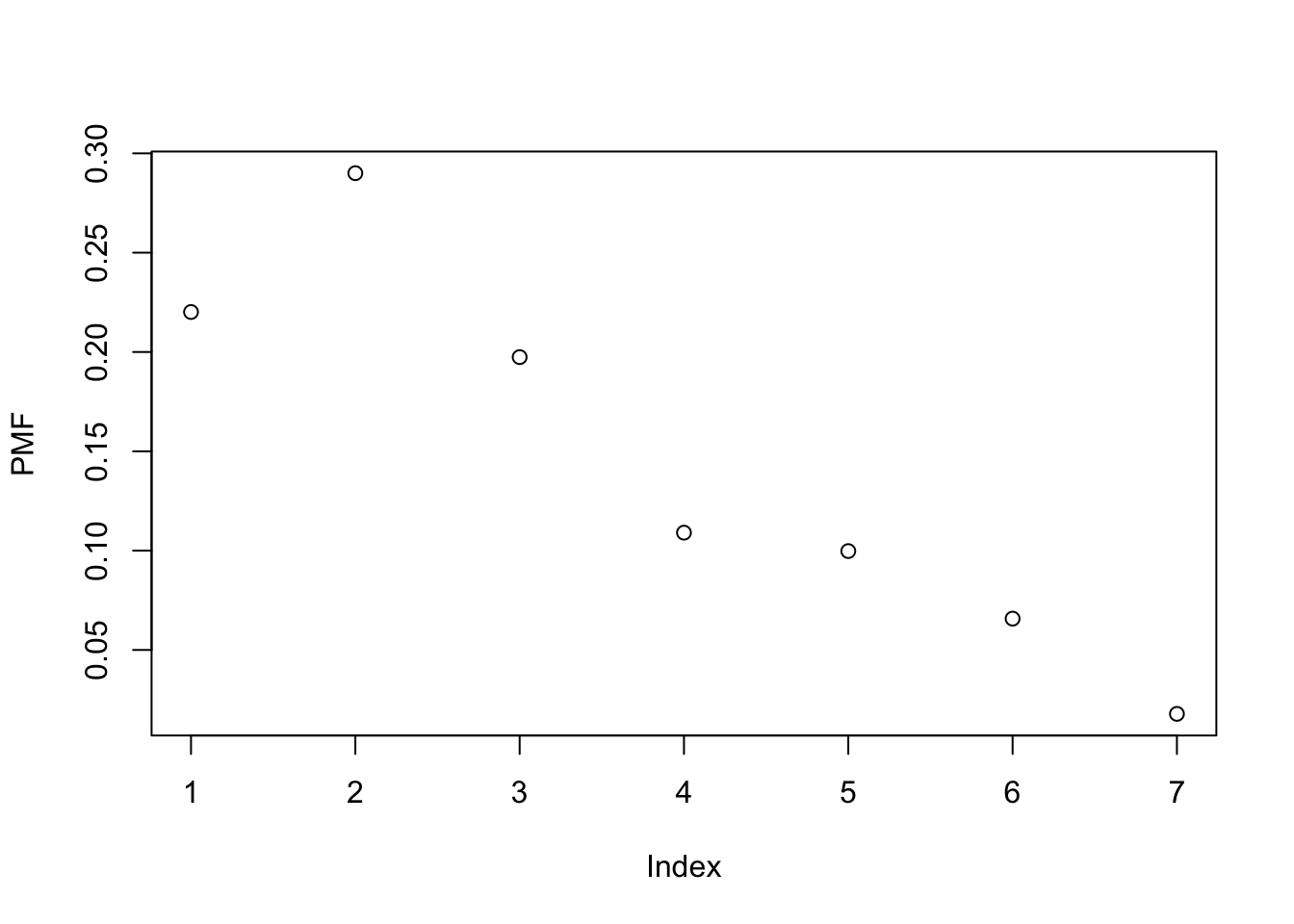
Looks like this is a valid PMF. Nice! We can also plot this.
plot(PMF)
Cool!
Also, let us note that the indexing our PMF vector, and subsequently our PMF plot, are off by one. This is due to the 1-based indexing in r, even though our first entry in our vector corresponds to the \(k=0\) case. So, for example the probability of getting 4 tails is
PMF[5]
[1] 0.09977824
Simulation
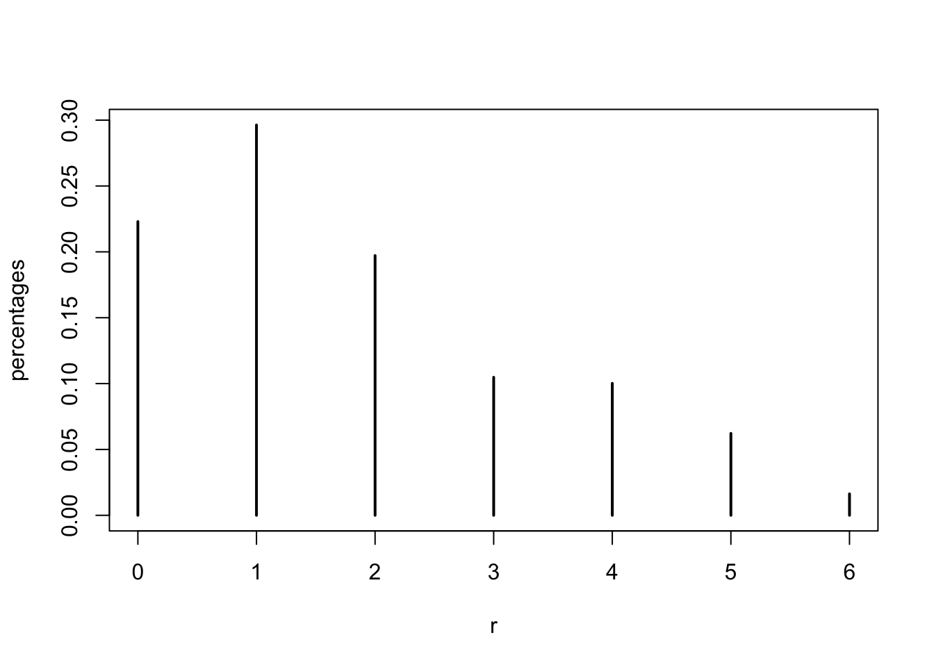
Now let us simulate our experiment to see if it matches our calculated PMF.
First, I will create some structures corresponding to my ingredients in R:
Now I write a function that will run the experiment:
Trials <-10^4# number of times to run the experiment; start with a small number for debuggingsimulate <-function() { # each call to simulate is one trial die =c(0,0,0,0,0,0) #Create an empty vector defining our die to manipulate later N = (sample(1:4,1,replace=FALSE)) #Sample a random number from 1 to 4 to simulate getting #one of the four suits from drawing a card#Assign die and coin accordingly based on card drawif(N ==1) { die = die_a coin = coin1; }if(N ==2) { die = die_b coin = coin2 }if(N ==3) { die = die_c coin = coin1; }if(N ==4) { die = die_d coin = coin2 } N = (sample(1:6,1,replace=FALSE,die)) # roll die#Loop through simulating coin flips based on the die roll. Count hte tails tails =0for(i in1:N) { if(runif(1)>coin) { tails = tails+1 } }return(tails)}r <-replicate(Trials,simulate()) # run experiment many times and store outcomes in a vector
percentages <-table(r)/Trials # tabulate frequencies of outcomespercentages