Analyzing the DC BikeShare System

Author

Irene Yank and Tristan Zook

Note

This technical report is accompanied by a plain-language report written to theoretical shareholders.

Introduction

We are investigating the bike sharing data set, which includes data on the Capital Bikeshare System, a bike rental service in Washington D.C. The main variable of interest in this data set is count, which represents the total number of bikes rented in a given day (There is also hourly data available, though daily data is used for the purpose of this project). After setting up feature engineering, we build and analyze several models and utilize cross validation to evaluate and compare the models. Once the optimal model is chosen, it is then used on the test set and further evaluated for its performance.

Data

# loading data
bike <- read.csv("day.csv")

# minor data cleaning
bike <- bike %>% 
    select(!c(instant,dteday, registered, casual,yr))

bike$weekday <- as.character(bike$weekday)
bike$season <- as.character(bike$season)
bike$mnth <- as.character(bike$mnth)

# task: predict 'cnt' (bike count) using necessary features

Our data comes from the UC Davis Machine Learning Repository and has 731 observations (2 years worth of data). Some features included the season, month, and different weather observations. All features used, along with their description and units if applicable are listed below:

Variable Name	Role	Description	Units
season	Feature	1:winter, 2:spring, 3:summer, 4:fall
month	Feature	month (1 to 12)
holiday	Feature	weather day is holiday or not (extracted from http://dchr.dc.gov/page/holiday-schedule)
weekday	Feature	day of the week
workingday	Feature	if day is neither weekend nor holiday is 1, otherwise is 0
weathersit	Feature	- 1: Clear, Few clouds, Partly cloudy, Partly cloudy
temp	Feature	Normalized temperature in Celsius. The values are derived via (t-t_min)/(t_max-t_min), t_min=-8, t_max=+39 (only in hourly scale)	C
atemp	Feature	Normalized feeling temperature in Celsius. The values are derived via (t-t_min)/(t_max-t_min), t_min=-16, t_max=+50 (only in hourly scale)	C
hum	Feature	Normalized humidity. The values are divided to 100 (max)
windspeed	Feature	Normalized wind speed. The values are divided to 67 (max)
count	Target	count of total rental bikes including both casual and registered

set.seed(208)

# data exploration

glimpse(bike)

Rows: 731
Columns: 11
$ season     <chr> "1", "1", "1", "1", "1", "1", "1", "1", "1", "1", "1", "1",…
$ mnth       <chr> "1", "1", "1", "1", "1", "1", "1", "1", "1", "1", "1", "1",…
$ holiday    <int> 0, 0, 0, 0, 0, 0, 0, 0, 0, 0, 0, 0, 0, 0, 0, 0, 1, 0, 0, 0,…
$ weekday    <chr> "6", "0", "1", "2", "3", "4", "5", "6", "0", "1", "2", "3",…
$ workingday <int> 0, 0, 1, 1, 1, 1, 1, 0, 0, 1, 1, 1, 1, 1, 0, 0, 0, 1, 1, 1,…
$ weathersit <int> 2, 2, 1, 1, 1, 1, 2, 2, 1, 1, 2, 1, 1, 1, 2, 1, 2, 2, 2, 2,…
$ temp       <dbl> 0.3441670, 0.3634780, 0.1963640, 0.2000000, 0.2269570, 0.20…
$ atemp      <dbl> 0.3636250, 0.3537390, 0.1894050, 0.2121220, 0.2292700, 0.23…
$ hum        <dbl> 0.805833, 0.696087, 0.437273, 0.590435, 0.436957, 0.518261,…
$ windspeed  <dbl> 0.1604460, 0.2485390, 0.2483090, 0.1602960, 0.1869000, 0.08…
$ cnt        <int> 985, 801, 1349, 1562, 1600, 1606, 1510, 959, 822, 1321, 126…

# numerical features: temp, atemp, hum, windspeed
  # step_normalize

# holiday and workingday are both categorical but already dummy encoded (1 indicates is is that type of day, 0 otherwise)

# weekday, month, and season are non-ordinal and categorical
  # step_dummy

# weathersit is ordinal -> 1 = clear, 2 = few clouds, 3 = partly cloudy, so it has already been step_integered for us

sum(is.na(bike))

[1] 0

# no NA values

Feature Engineering

set.seed(208)

# data splitting

data_split <- initial_split(data = bike, prop = 0.8)

bike_train <- training(data_split)  

bike_test <- testing(data_split)

set.seed(208)

nearZeroVar(bike_train, saveMetrics = TRUE)

           freqRatio percentUnique zeroVar   nzv
season      1.013423     0.6849315   FALSE FALSE
mnth        1.019231     2.0547945   FALSE FALSE
holiday    33.352941     0.3424658   FALSE  TRUE
weekday     1.011494     1.1986301   FALSE FALSE
workingday  2.173913     0.3424658   FALSE FALSE
weathersit  1.912821     0.5136986   FALSE FALSE
temp        1.250000    71.4041096   FALSE FALSE
atemp       1.333333    94.5205479   FALSE FALSE
hum         1.333333    84.0753425   FALSE FALSE
windspeed   1.000000    91.0958904   FALSE FALSE
cnt         1.000000    96.4041096   FALSE FALSE

# holiday is nzv, which should make sense there aren't a ton of holidays, still seems like it could be an important feature to include

set.seed(208)

# feature engineering (full)

bike_recipe <- recipe(formula = cnt ~., data = bike_train)

bike_blueprint <- bike_recipe %>%    
  step_normalize(temp, atemp, hum, windspeed) %>%
  step_dummy(weekday, mnth, season, one_hot = FALSE)                

bike_prepare <- prep(bike_blueprint, data = bike_train)    

bike_baked_train <- bake(bike_prepare, new_data = bike_train)   

bike_baked_test <- bake(bike_prepare, new_data = bike_test)

# check baked dataset 

glimpse(bike_baked_train)

Rows: 584
Columns: 28
$ holiday    <int> 0, 0, 0, 0, 0, 0, 0, 0, 0, 0, 0, 0, 0, 0, 0, 0, 0, 0, 1, 0,…
$ workingday <int> 1, 0, 0, 1, 1, 1, 0, 1, 1, 1, 1, 1, 1, 1, 1, 1, 0, 1, 0, 1,…
$ weathersit <int> 1, 1, 2, 1, 2, 2, 1, 2, 1, 1, 1, 1, 1, 1, 2, 1, 2, 1, 1, 1,…
$ temp       <dbl> 0.8492669, 0.6474146, -0.4673502, 1.5052771, -0.2976142, 0.…
$ atemp      <dbl> 0.7676468, 0.6896242, -0.3757399, 1.6884675, -0.2665057, 0.…
$ hum        <dbl> -1.1173994, -0.3498378, 0.9077861, 0.5771409, 0.9373102, 0.…
$ windspeed  <dbl> -0.19277865, 0.45412663, 1.32794434, -0.99358636, 1.8941392…
$ cnt        <int> 7736, 6118, 2429, 4332, 2566, 4727, 1787, 1650, 4169, 6207,…
$ weekday_X1 <dbl> 0, 0, 0, 0, 0, 0, 0, 0, 0, 0, 0, 0, 0, 0, 0, 0, 0, 0, 1, 0,…
$ weekday_X2 <dbl> 0, 0, 0, 0, 0, 0, 0, 0, 0, 0, 1, 1, 1, 0, 1, 0, 0, 1, 0, 0,…
$ weekday_X3 <dbl> 0, 0, 0, 1, 1, 0, 0, 1, 1, 0, 0, 0, 0, 0, 0, 0, 0, 0, 0, 0,…
$ weekday_X4 <dbl> 0, 0, 0, 0, 0, 0, 0, 0, 0, 0, 0, 0, 0, 1, 0, 0, 0, 0, 0, 0,…
$ weekday_X5 <dbl> 1, 0, 0, 0, 0, 1, 0, 0, 0, 1, 0, 0, 0, 0, 0, 1, 0, 0, 0, 1,…
$ weekday_X6 <dbl> 0, 0, 1, 0, 0, 0, 0, 0, 0, 0, 0, 0, 0, 0, 0, 0, 0, 0, 0, 0,…
$ mnth_X10   <dbl> 0, 0, 1, 0, 0, 0, 0, 0, 0, 0, 0, 0, 0, 0, 1, 0, 0, 0, 0, 0,…
$ mnth_X11   <dbl> 0, 0, 0, 0, 1, 0, 0, 0, 0, 0, 0, 0, 0, 0, 0, 0, 0, 0, 0, 1,…
$ mnth_X12   <dbl> 0, 0, 0, 0, 0, 0, 1, 0, 0, 0, 0, 0, 0, 0, 0, 0, 0, 0, 0, 0,…
$ mnth_X2    <dbl> 0, 0, 0, 0, 0, 0, 0, 0, 1, 0, 0, 0, 0, 0, 0, 0, 1, 0, 1, 0,…
$ mnth_X3    <dbl> 0, 0, 0, 0, 0, 0, 0, 0, 0, 0, 0, 0, 0, 1, 0, 0, 0, 0, 0, 0,…
$ mnth_X4    <dbl> 0, 0, 0, 0, 0, 0, 0, 0, 0, 0, 0, 0, 0, 0, 0, 0, 0, 0, 0, 0,…
$ mnth_X5    <dbl> 0, 1, 0, 0, 0, 0, 0, 0, 0, 0, 1, 0, 0, 0, 0, 0, 0, 0, 0, 0,…
$ mnth_X6    <dbl> 1, 0, 0, 0, 0, 0, 0, 0, 0, 0, 0, 0, 0, 0, 0, 0, 0, 0, 0, 0,…
$ mnth_X7    <dbl> 0, 0, 0, 1, 0, 0, 0, 0, 0, 1, 0, 0, 1, 0, 0, 1, 0, 0, 0, 0,…
$ mnth_X8    <dbl> 0, 0, 0, 0, 0, 0, 0, 0, 0, 0, 0, 1, 0, 0, 0, 0, 0, 0, 0, 0,…
$ mnth_X9    <dbl> 0, 0, 0, 0, 0, 1, 0, 0, 0, 0, 0, 0, 0, 0, 0, 0, 0, 1, 0, 0,…
$ season_X2  <dbl> 1, 1, 0, 0, 0, 0, 0, 0, 0, 0, 1, 0, 0, 1, 0, 0, 0, 0, 0, 0,…
$ season_X3  <dbl> 0, 0, 0, 1, 0, 1, 0, 0, 0, 1, 0, 1, 1, 0, 0, 1, 0, 1, 0, 0,…
$ season_X4  <dbl> 0, 0, 1, 0, 1, 0, 0, 0, 0, 0, 0, 0, 0, 0, 1, 0, 0, 0, 0, 1,…

summary(bike_baked_train)

    holiday          workingday       weathersit         temp         
 Min.   :0.00000   Min.   :0.0000   Min.   :1.000   Min.   :-2.39889  
 1st Qu.:0.00000   1st Qu.:0.0000   1st Qu.:1.000   1st Qu.:-0.87793  
 Median :0.00000   Median :1.0000   Median :1.000   Median : 0.02351  
 Mean   :0.02911   Mean   :0.6849   Mean   :1.389   Mean   : 0.00000  
 3rd Qu.:0.00000   3rd Qu.:1.0000   3rd Qu.:2.000   3rd Qu.: 0.87220  
 Max.   :1.00000   Max.   :1.0000   Max.   :3.000   Max.   : 2.01908  
     atemp               hum             windspeed            cnt      
 Min.   :-2.43875   Min.   :-4.43269   Min.   :-2.1828   Min.   :  22  
 1st Qu.:-0.85760   1st Qu.:-0.77347   1st Qu.:-0.7266   1st Qu.:3212  
 Median : 0.08472   Median :-0.01477   Median :-0.1363   Median :4540  
 Mean   : 0.00000   Mean   : 0.00000   Mean   : 0.0000   Mean   :4515  
 3rd Qu.: 0.83009   3rd Qu.: 0.73435   3rd Qu.: 0.5697   3rd Qu.:5978  
 Max.   : 2.26972   Max.   : 2.45767   Max.   : 4.1267   Max.   :8714  
   weekday_X1       weekday_X2       weekday_X3       weekday_X4    
 Min.   :0.0000   Min.   :0.0000   Min.   :0.0000   Min.   :0.0000  
 1st Qu.:0.0000   1st Qu.:0.0000   1st Qu.:0.0000   1st Qu.:0.0000  
 Median :0.0000   Median :0.0000   Median :0.0000   Median :0.0000  
 Mean   :0.1507   Mean   :0.1421   Mean   :0.1404   Mean   :0.1353  
 3rd Qu.:0.0000   3rd Qu.:0.0000   3rd Qu.:0.0000   3rd Qu.:0.0000  
 Max.   :1.0000   Max.   :1.0000   Max.   :1.0000   Max.   :1.0000  
   weekday_X5       weekday_X6       mnth_X10          mnth_X11      
 Min.   :0.0000   Min.   :0.000   Min.   :0.00000   Min.   :0.00000  
 1st Qu.:0.0000   1st Qu.:0.000   1st Qu.:0.00000   1st Qu.:0.00000  
 Median :0.0000   Median :0.000   Median :0.00000   Median :0.00000  
 Mean   :0.1455   Mean   :0.137   Mean   :0.08733   Mean   :0.09075  
 3rd Qu.:0.0000   3rd Qu.:0.000   3rd Qu.:0.00000   3rd Qu.:0.00000  
 Max.   :1.0000   Max.   :1.000   Max.   :1.00000   Max.   :1.00000  
    mnth_X12         mnth_X2           mnth_X3           mnth_X4       
 Min.   :0.0000   Min.   :0.00000   Min.   :0.00000   Min.   :0.00000  
 1st Qu.:0.0000   1st Qu.:0.00000   1st Qu.:0.00000   1st Qu.:0.00000  
 Median :0.0000   Median :0.00000   Median :0.00000   Median :0.00000  
 Mean   :0.0839   Mean   :0.08048   Mean   :0.07534   Mean   :0.08904  
 3rd Qu.:0.0000   3rd Qu.:0.00000   3rd Qu.:0.00000   3rd Qu.:0.00000  
 Max.   :1.0000   Max.   :1.00000   Max.   :1.00000   Max.   :1.00000  
    mnth_X5           mnth_X6          mnth_X7           mnth_X8       
 Min.   :0.00000   Min.   :0.0000   Min.   :0.00000   Min.   :0.00000  
 1st Qu.:0.00000   1st Qu.:0.0000   1st Qu.:0.00000   1st Qu.:0.00000  
 Median :0.00000   Median :0.0000   Median :0.00000   Median :0.00000  
 Mean   :0.08733   Mean   :0.0839   Mean   :0.08219   Mean   :0.07705  
 3rd Qu.:0.00000   3rd Qu.:0.0000   3rd Qu.:0.00000   3rd Qu.:0.00000  
 Max.   :1.00000   Max.   :1.0000   Max.   :1.00000   Max.   :1.00000  
    mnth_X9          season_X2        season_X3      season_X4     
 Min.   :0.00000   Min.   :0.0000   Min.   :0.00   Min.   :0.0000  
 1st Qu.:0.00000   1st Qu.:0.0000   1st Qu.:0.00   1st Qu.:0.0000  
 Median :0.00000   Median :0.0000   Median :0.00   Median :0.0000  
 Mean   :0.08562   Mean   :0.2586   Mean   :0.25   Mean   :0.2551  
 3rd Qu.:0.00000   3rd Qu.:1.0000   3rd Qu.:0.25   3rd Qu.:1.0000  
 Max.   :1.00000   Max.   :1.0000   Max.   :1.00   Max.   :1.0000

Minimal Feature Engineering

set.seed(208)

# feature engineering (minimal)

bike_recipe <- recipe(formula = cnt ~., data = bike_train)

bike_blueprint_min <- bike_recipe               

bike_prepare_min <- prep(bike_blueprint_min, data = bike_train)    

bike_baked_train_min <- bake(bike_prepare_min, new_data = bike_train)   

bike_baked_test_min <- bake(bike_prepare_min, new_data = bike_test)

Analysis/Methodology

We did some initial data exploration, looking in to the types of variables present, ranges of values for variables, any missing entries, etc. There were some variables we decided to remove from our dataset prior to model building for a number of reasons. For example, we removed the yr and date variables as these do not provide any helpful information for future predictions, and we would not want them influencing our model. We found no missing entries in the variables we will use. The only feature engineering we found it necessary to implement was normalizing numeric predictors and dummy encoding categorical predictors. We also created a minimal FE blueprint with no feature engineering to test applicable models on this as well. We considered an 80-20 split for splitting our data and creating training and test sets.

This is a supervised, regression problem so a logistic regression would not make sense to use in this case. Instead, we will build and compare the following models:

Linear Regression
KNN
Single Tree
Random Forest
Boosted Trees

All of these models besides KNN will be built on both the full feature engineered training data, as well as the minimal FE data. Minimal feature engineering only includes imputing missing values, and since we have none of those, the models will simply be trained and tested on the original training and test sets. All models will be trained and compared using the CV process to tune hyperparameters and obtain test predictions for accuracy.

# CV specifications

set.seed(208)

cv_specs_bike <- trainControl(method = "repeatedcv",    # CV method
                         number = 5,              # number of folds
                         repeats = 1)              # number of repeats

# for KNN

k_grid_bike <- expand.grid(k = seq(1, 51, by = 10))

# for random forests

param_grid_rf_bike <- expand.grid(mtry = seq(1, 10, 1),    
                                   splitrule = "variance",
                                   min.node.size = 2)

set.seed(208)

# linear (full FE)

lm_cv_bike <- train(bike_blueprint,
                         data = bike_train,
                         method = "lm",
                         trControl = cv_specs_bike,
                         metric = "RMSE")

set.seed(208)

# linear (min FE)

lm_cv_bike_min <- train(bike_blueprint_min,
                         data = bike_train,
                         method = "lm",
                         trControl = cv_specs_bike,
                         metric = "RMSE")

set.seed(208)

# KNN 

knn_cv_bike <- train(bike_blueprint,
                data = bike_train, 
                method = "knn",
                trControl = cv_specs_bike,
                tuneGrid = k_grid_bike,
                metric = "RMSE")

set.seed(208)

# tree (full FE)

tree_cv_bike <- train(bike_blueprint,
                        data = bike_train,
                        method = "rpart",  
                        trControl = cv_specs_bike,
                        tuneLength = 20,                   
                        metric = "RMSE")

set.seed(208)

# tree (min FE)

tree_cv_bike_min <- train(bike_blueprint_min,
                        data = bike_train,
                        method = "rpart",  
                        trControl = cv_specs_bike,
                        tuneLength = 20,                   
                        metric = "RMSE")

set.seed(208)

# random forest (full FE)

rf_cv_bike <- train(bike_blueprint,
               data = bike_train,
               method = "ranger",
               trControl = cv_specs_bike,
               tuneGrid = param_grid_rf_bike,
               metric = "RMSE")

set.seed(208)

# random forest (min FE)

rf_cv_bike_min <- train(bike_blueprint_min,
               data = bike_train,
               method = "ranger",
               trControl = cv_specs_bike,
               tuneGrid = param_grid_rf_bike,
               metric = "RMSE")

set.seed(208)

# gradient boosting (full FE)

out_bike <- capture.output(
  gbm_cv_bike <- train(bike_blueprint,
                  data = bike_train,
                  method = "gbm",  
                  trControl = cv_specs_bike,
                  tuneLength = 5,
                  metric = "RMSE"))

set.seed(208)

# gradient boosting (min FE) 

out_bike_min <- capture.output(
  gbm_cv_bike_min <- train(bike_blueprint_min,
                  data = bike_train,
                  method = "gbm",  
                  trControl = cv_specs_bike,
                  tuneLength = 5,
                  metric = "RMSE"))

CV Results

RMSE

set.seed(208)

# optimal RMSE

min(lm_cv_bike$results$RMSE)

[1] 1353.256

min(lm_cv_bike_min$results$RMSE)

[1] 1353.256

min(knn_cv_bike$results$RMSE)

[1] 1259.461

min(tree_cv_bike$results$RMSE)

[1] 1393.776

min(tree_cv_bike_min$results$RMSE)

[1] 1399.762

min(rf_cv_bike$results$RMSE)

[1] 1246.361

min(rf_cv_bike_min$results$RMSE)

[1] 1241.927

min(gbm_cv_bike$results$RMSE)

[1] 1255.633

min(gbm_cv_bike_min$results$RMSE)

[1] 1346.863

RMSE SD

set.seed(208)

# RMSESD

lm_cv_bike$results$RMSESD[which.min(lm_cv_bike$results$RMSE)]

[1] 66.96529

lm_cv_bike_min$results$RMSESD[which.min(lm_cv_bike_min$results$RMSE)]

[1] 66.96529

knn_cv_bike$results$RMSESD[which.min(knn_cv_bike$results$RMSE)]

[1] 66.39121

tree_cv_bike$results$RMSESD[which.min(tree_cv_bike$results$RMSE)]

[1] 108.2552

tree_cv_bike_min$results$RMSESD[which.min(tree_cv_bike_min$results$RMSE)]

[1] 108.4535

rf_cv_bike$results$RMSESD[which.min(rf_cv_bike$results$RMSE)]

[1] 69.62765

rf_cv_bike_min$results$RMSESD[which.min(rf_cv_bike_min$results$RMSE)]

[1] 63.96872

gbm_cv_bike$results$RMSESD[which.min(gbm_cv_bike$results$RMSE)]

[1] 67.95094

gbm_cv_bike_min$results$RMSESD[which.min(gbm_cv_bike_min$results$RMSE)]

[1] 73.97493

Optimal Parameters

set.seed(208)

# best tune 

knn_cv_bike$bestTune

   k
3 21

tree_cv_bike$bestTune

            cp
12 0.009757784

tree_cv_bike_min$bestTune

           cp
14 0.01449829

rf_cv_bike$bestTune

  mtry splitrule min.node.size
8    8  variance             2

rf_cv_bike_min$bestTune

  mtry splitrule min.node.size
2    2  variance             2

gbm_cv_bike$bestTune

  n.trees interaction.depth shrinkage n.minobsinnode
7     100                 2       0.1             10

gbm_cv_bike_min$bestTune

  n.trees interaction.depth shrinkage n.minobsinnode
6      50                 2       0.1             10

Results

The following table gives the concise results of our CV:

Technique	RMSE	RMSE SD	Optimal Parameters
LM (Full FE)	1353.256	66.96529	-
LM (Min FE)	1353.256	66.96529	-
KNN (Full FE)	1259.461	66.39121	k = 21
Tree (Full FE)	1393.776	108.2552	cp = 0.00976
Tree (Min FE)	1399.762	108.4535	cp = 0.0145
Random Forest (Full FE)	1246.416	73.35131	mtry = 6
Random Forest (Min FE)	1239.478	62.84000	mtry = 3
Gradient Boosting (Full FE)	1255.566	70.53906	100 - 2 - 0.1 - 10
Gradient Boosting (Min FE)	1348.092	74.03074	250 - 1 - 0.1 - 10

The Random Forest with minimal FE has the lowest training loss at 1239.478, along with the lowest RMSE SD at 62.84. Not only does it seem to provide a good fit for the data, but it does not come at the cost of increased variability. For these reasons, we chose this model as the final model to use on the test set and for future data.

Final Model

set.seed(208)

# Random Forest (Min FE) is our optimal model in training. We train it here and report test RMSE.

final_model_bike <- ranger(formula = cnt ~ .,
                      data = bike_baked_train_min,
                      num.trees = 500,
                      mtry = rf_cv_bike_min$bestTune$mtry,
                      splitrule = "variance",
                      min.node.size = 2,
                      importance = "impurity")

final_model_preds_bike <- predict(object = final_model_bike, data = bike_baked_test_min, type = "response")  

sqrt(mean((final_model_preds_bike$predictions - bike_baked_test_min$cnt)^2))

[1] 1168.83

# if implemented on a new dataset, we are likely to see an error around 1159.892

# check VIPs
set.seed(208)

vip(final_model_bike, num_features = 10)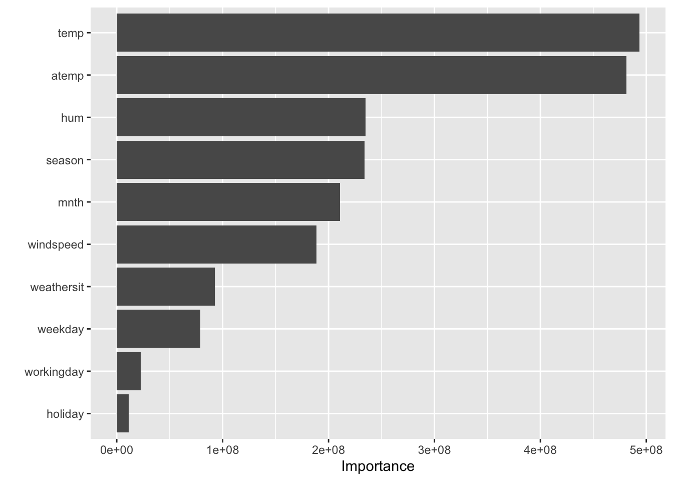

# The top 3 VIP's are temp, atemp, and humidity. These seem to make sense logically, and we can maybe assume correlation ourselves. For example, warmer weather most likely correlates with more bikes rented. However, our model cannot tell us the nature of the specific relationship between these variables and our response of count.

Conclusion

After performing cross validation to tune hyperparameters and compare training performance across all tested models, we found the optimal model to be the random forested implemented with minimal FE, and mtry=3. On the training set, this model yielded an RMSE of 1240 and RMSESD of 63. When training the final model, and using it to predict on our test set, we found an RMSE of around 1160.

When checking our VIP’s, we see the variables that influence our predictions the most are temperature, average temperature, and humidity. These may be expected. However, our model cannot give us any additional information about specifically how these variables influence prediction.

The random forest with minimal FE seems to be the optimal model on all accounts. Any others that are close to its performance would not add any additional interpretability, usefulness, or reduction in computation power. If we were looking for more interpretability or less resources used, we could perhaps train the linear model with no feature engineering. While this did perform outright worse than the random forest, its interpretability and minmimal computation power needed could make it useful in application.