Mountaineering Data Analysis with SQL

The second project in CMSC405 involved making use of SQL+R to design and create a relational database with at least three different datasets that could be joined with a common key, and then perform data analysis on our database. My partner Laura Henze and I chose to investigate Himalayan Mountaineering data. Find our database creation and exploration below.

Accessing data

We will be considering the Himalayan Climbing Expedition datasets available on GitHub. Himalayan Expedition Datasets

Create the connection

con_exp <- DBI::dbConnect(duckdb::duckdb(), dbdir = "exp_db")

duckdb keeps downloaded extensions and secrets in a temporary directory:
ℹ /var/folders/yw/z7lhcw3n4ddblqzq_7hp9dm80000gn/T//Rtmpbe8M96/duckdb
This is removed when the R session ends.
• Extensions are re-downloaded each session.
• Secrets are lost.
ℹ Run duckdb(shared_home = TRUE) (or create ~/.duckdb) to keep them (suitable for most users).
ℹ Run duckdb(shared_home = FALSE) to accept the temporary directory (and silence this message).
ℹ See ?duckdb_storage for details and alternatives.

Read in the raw data from Github

members <- readr::read_csv('https://raw.githubusercontent.com/rfordatascience/tidytuesday/main/data/2020/2020-09-22/members.csv')

Rows: 76519 Columns: 21
── Column specification ────────────────────────────────────────────────────────
Delimiter: ","
chr (10): expedition_id, member_id, peak_id, peak_name, season, sex, citizen...
dbl  (5): year, age, highpoint_metres, death_height_metres, injury_height_me...
lgl  (6): hired, success, solo, oxygen_used, died, injured

ℹ Use `spec()` to retrieve the full column specification for this data.
ℹ Specify the column types or set `show_col_types = FALSE` to quiet this message.

expeditions <- readr::read_csv('https://raw.githubusercontent.com/rfordatascience/tidytuesday/main/data/2020/2020-09-22/expeditions.csv')

Rows: 10364 Columns: 16
── Column specification ────────────────────────────────────────────────────────
Delimiter: ","
chr  (6): expedition_id, peak_id, peak_name, season, termination_reason, tre...
dbl  (6): year, highpoint_metres, members, member_deaths, hired_staff, hired...
lgl  (1): oxygen_used
date (3): basecamp_date, highpoint_date, termination_date

ℹ Use `spec()` to retrieve the full column specification for this data.
ℹ Specify the column types or set `show_col_types = FALSE` to quiet this message.

peaks <- readr::read_csv('https://raw.githubusercontent.com/rfordatascience/tidytuesday/main/data/2020/2020-09-22/peaks.csv')

Rows: 468 Columns: 8
── Column specification ────────────────────────────────────────────────────────
Delimiter: ","
chr (6): peak_id, peak_name, peak_alternative_name, climbing_status, first_a...
dbl (2): height_metres, first_ascent_year

ℹ Use `spec()` to retrieve the full column specification for this data.
ℹ Specify the column types or set `show_col_types = FALSE` to quiet this message.

glimpse(peaks)

Rows: 468
Columns: 8
$ peak_id                    <chr> "AMAD", "AMPG", "ANN1", "ANN2", "ANN3", "AN…
$ peak_name                  <chr> "Ama Dablam", "Amphu Gyabjen", "Annapurna I…
$ peak_alternative_name      <chr> "Amai Dablang", NA, NA, NA, NA, NA, NA, NA,…
$ height_metres              <dbl> 6814, 5630, 8091, 7937, 7555, 7525, 8026, 8…
$ climbing_status            <chr> "Climbed", "Climbed", "Climbed", "Climbed",…
$ first_ascent_year          <dbl> 1961, 1953, 1950, 1960, 1961, 1955, 1974, 1…
$ first_ascent_country       <chr> "New Zealand, USA, UK", "UK", "France", "UK…
$ first_ascent_expedition_id <chr> "AMAD61101", "AMPG53101", "ANN150101", "ANN…

# Quick check to see what the data look like

summary(peaks)

      peak_id        peak_name   peak_alternative_name height_metres 
 Length   :468   Length   :468   Length   :468         Min.   :5407  
 N.unique :468   N.unique :468   N.unique :242         1st Qu.:6236  
 N.blank  :  0   N.blank  :  0   N.blank  :  0         Median :6560  
 Min.nchar:  4   Min.nchar:  4   Min.nchar:  5         Mean   :6657  
 Max.nchar:  4   Max.nchar: 25   Max.nchar: 49         3rd Qu.:6911  
                                 NAs      :223         Max.   :8850  
                                                                     
  climbing_status first_ascent_year first_ascent_country
 Length   :468    Min.   : 201      Length   :468       
 N.unique :  2    1st Qu.:1963      N.unique : 77       
 N.blank  :  0    Median :1982      N.blank  :  0       
 Min.nchar:  7    Mean   :1979      Min.nchar:  2       
 Max.nchar:  9    3rd Qu.:2008      Max.nchar: 44       
                  Max.   :2019      NAs      :132       
                  NAs    :132                           
 first_ascent_expedition_id
 Length   :468             
 N.unique :332             
 N.blank  :  0             
 Min.nchar:  9             
 Max.nchar:  9             
 NAs      :135             
                           

# Nothing seems like it needs to be removed.

glimpse(expeditions)

Rows: 10,364
Columns: 16
$ expedition_id      <chr> "ANN260101", "ANN269301", "ANN273101", "ANN278301",…
$ peak_id            <chr> "ANN2", "ANN2", "ANN2", "ANN2", "ANN2", "ANN2", "AN…
$ peak_name          <chr> "Annapurna II", "Annapurna II", "Annapurna II", "An…
$ year               <dbl> 1960, 1969, 1973, 1978, 1979, 1980, 1980, 1981, 198…
$ season             <chr> "Spring", "Autumn", "Spring", "Autumn", "Autumn", "…
$ basecamp_date      <date> 1960-03-15, 1969-09-25, 1973-03-16, 1978-09-08, NA…
$ highpoint_date     <date> 1960-05-17, 1969-10-22, 1973-05-06, 1978-10-02, 19…
$ termination_date   <date> NA, 1969-10-26, NA, 1978-10-05, 1979-10-20, 1980-0…
$ termination_reason <chr> "Success (main peak)", "Success (main peak)", "Succ…
$ highpoint_metres   <dbl> 7937, 7937, 7937, 7000, 7160, 7000, 7250, 6400, 740…
$ members            <dbl> 10, 10, 6, 2, 3, 6, 7, 19, 9, 5, 5, 5, 6, 4, 3, 4, …
$ member_deaths      <dbl> 0, 0, 0, 0, 0, 1, 0, 0, 1, 0, 1, 0, 0, 0, 0, 0, 0, …
$ hired_staff        <dbl> 9, 0, 8, 0, 0, 2, 2, 0, 3, 0, 0, 3, 4, 2, 0, 2, 5, …
$ hired_staff_deaths <dbl> 0, 0, 0, 0, 0, 0, 0, 0, 0, 0, 0, 0, 0, 0, 0, 0, 0, …
$ oxygen_used        <lgl> TRUE, FALSE, FALSE, FALSE, FALSE, FALSE, FALSE, FAL…
$ trekking_agency    <chr> NA, NA, NA, NA, NA, NA, NA, NA, NA, NA, NA, "Kunga"…

# Quick check to see what the data look like

summary(expeditions)

   expedition_id        peak_id          peak_name          year     
 Length   :10364   Length   :10364   Length   :10364   Min.   :1905  
 N.unique :10363   N.unique :  391   N.unique :  390   1st Qu.:1994  
 N.blank  :    0   N.blank  :    0   N.blank  :    0   Median :2005  
 Min.nchar:    9   Min.nchar:    4   Min.nchar:    4   Mean   :2001  
 Max.nchar:    9   Max.nchar:    4   Max.nchar:   25   3rd Qu.:2012  
                                     NAs      :    1   Max.   :2019  
                                                                     
       season      basecamp_date        highpoint_date      
 Length   :10364   Min.   :1921-06-26   Min.   :1905-09-01  
 N.unique :    5   1st Qu.:1994-11-25   1st Qu.:1995-02-03  
 N.blank  :    0   Median :2005-04-15   Median :2005-09-26  
 Min.nchar:    6   Mean   :2002-02-19   Mean   :2002-04-09  
 Max.nchar:    7   3rd Qu.:2011-05-15   3rd Qu.:2011-11-16  
                   Max.   :2019-05-27   Max.   :2019-05-30  
                   NAs    :1095         NAs    :650         
 termination_date     termination_reason highpoint_metres    members      
 Min.   :1921-09-30   Length   :10364    Min.   :3500     Min.   : 0.000  
 1st Qu.:1998-10-19   N.unique :   15    1st Qu.:6700     1st Qu.: 2.000  
 Median :2006-10-03   N.blank  :    0    Median :7300     Median : 5.000  
 Mean   :2004-01-06   Min.nchar:    5    Mean   :7409     Mean   : 5.953  
 3rd Qu.:2012-05-07   Max.nchar:   76    3rd Qu.:8188     3rd Qu.: 8.000  
 Max.   :2019-06-04                      Max.   :8850     Max.   :99.000  
 NAs    :2380                            NAs    :414                      
 member_deaths       hired_staff     hired_staff_deaths oxygen_used    
 Min.   : 0.00000   Min.   : 0.000   Min.   : 0.00000   Mode :logical  
 1st Qu.: 0.00000   1st Qu.: 0.000   1st Qu.: 0.00000   FALSE:7452     
 Median : 0.00000   Median : 1.000   Median : 0.00000   TRUE :2912     
 Mean   : 0.07603   Mean   : 2.777   Mean   : 0.03068                  
 3rd Qu.: 0.00000   3rd Qu.: 3.000   3rd Qu.: 0.00000                  
 Max.   :10.00000   Max.   :99.000   Max.   :11.00000                  
                                                                       
  trekking_agency 
 Length   :10364  
 N.unique :  828  
 N.blank  :    0  
 Min.nchar:    4  
 Max.nchar:   50  
 NAs      : 1580  
                  

#Don't see any issue in keeping everything for now, besides peak_name 
# which will be redundant after join.

glimpse(members)

Rows: 76,519
Columns: 21
$ expedition_id        <chr> "AMAD78301", "AMAD78301", "AMAD78301", "AMAD78301…
$ member_id            <chr> "AMAD78301-01", "AMAD78301-02", "AMAD78301-03", "…
$ peak_id              <chr> "AMAD", "AMAD", "AMAD", "AMAD", "AMAD", "AMAD", "…
$ peak_name            <chr> "Ama Dablam", "Ama Dablam", "Ama Dablam", "Ama Da…
$ year                 <dbl> 1978, 1978, 1978, 1978, 1978, 1978, 1978, 1978, 1…
$ season               <chr> "Autumn", "Autumn", "Autumn", "Autumn", "Autumn",…
$ sex                  <chr> "M", "M", "M", "M", "M", "M", "M", "M", "M", "M",…
$ age                  <dbl> 40, 41, 27, 40, 34, 25, 41, 29, 35, 37, 23, 44, 2…
$ citizenship          <chr> "France", "France", "France", "France", "France",…
$ expedition_role      <chr> "Leader", "Deputy Leader", "Climber", "Exp Doctor…
$ hired                <lgl> FALSE, FALSE, FALSE, FALSE, FALSE, FALSE, FALSE, …
$ highpoint_metres     <dbl> NA, 6000, NA, 6000, NA, 6000, 6000, 6000, NA, 681…
$ success              <lgl> FALSE, FALSE, FALSE, FALSE, FALSE, FALSE, FALSE, …
$ solo                 <lgl> FALSE, FALSE, FALSE, FALSE, FALSE, FALSE, FALSE, …
$ oxygen_used          <lgl> FALSE, FALSE, FALSE, FALSE, FALSE, FALSE, FALSE, …
$ died                 <lgl> FALSE, FALSE, FALSE, FALSE, FALSE, FALSE, FALSE, …
$ death_cause          <chr> NA, NA, NA, NA, NA, NA, NA, NA, NA, NA, NA, NA, N…
$ death_height_metres  <dbl> NA, NA, NA, NA, NA, NA, NA, NA, NA, NA, NA, NA, N…
$ injured              <lgl> FALSE, FALSE, FALSE, FALSE, FALSE, FALSE, FALSE, …
$ injury_type          <chr> NA, NA, NA, NA, NA, NA, NA, NA, NA, NA, NA, NA, N…
$ injury_height_metres <dbl> NA, NA, NA, NA, NA, NA, NA, NA, NA, NA, NA, NA, N…

# Quick check to see what the data look like

summary(members)

   expedition_id       member_id          peak_id          peak_name    
 Length   :76519   Length   :76519   Length   :76519   Length   :76519  
 N.unique :10350   N.unique :76518   N.unique :  391   N.unique :  390  
 N.blank  :    0   N.blank  :    0   N.blank  :    0   N.blank  :    0  
 Min.nchar:    9   Min.nchar:   12   Min.nchar:    4   Min.nchar:    4  
 Max.nchar:    9   Max.nchar:   12   Max.nchar:    4   Max.nchar:   25  
                                                       NAs      :   15  
                                                                        
      year            season             sex             age       
 Min.   :1905   Length   :76519   Length   :76519   Min.   : 7.00  
 1st Qu.:1991   N.unique :    5   N.unique :    2   1st Qu.:29.00  
 Median :2004   N.blank  :    0   N.blank  :    0   Median :36.00  
 Mean   :2000   Min.nchar:    6   Min.nchar:    1   Mean   :37.33  
 3rd Qu.:2012   Max.nchar:    7   Max.nchar:    1   3rd Qu.:44.00  
 Max.   :2019                     NAs      :    2   Max.   :85.00  
                                                    NAs    :3497   
    citizenship     expedition_role    hired         highpoint_metres
 Length   :76519   Length   :76519   Mode :logical   Min.   :3800    
 N.unique :  212   N.unique :  524   FALSE:60788     1st Qu.:6700    
 N.blank  :    0   N.blank  :    0   TRUE :15731     Median :7400    
 Min.nchar:    2   Min.nchar:    4                   Mean   :7471    
 Max.nchar:   23   Max.nchar:   25                   3rd Qu.:8400    
 NAs      :   10   NAs      :   21                   Max.   :8850    
                                                     NAs    :21833   
  success           solo         oxygen_used        died        
 Mode :logical   Mode :logical   Mode :logical   Mode :logical  
 FALSE:47320     FALSE:76398     FALSE:58286     FALSE:75413    
 TRUE :29199     TRUE :121       TRUE :18233     TRUE :1106     
                                                                
                                                                
                                                                
                                                                
    death_cause    death_height_metres  injured           injury_type   
 Length   :76519   Min.   : 400        Mode :logical   Length   :76519  
 N.unique :   12   1st Qu.:5800        FALSE:74806     N.unique :   11  
 N.blank  :    0   Median :6600        TRUE :1713      N.blank  :    0  
 Min.nchar:    3   Mean   :6593                        Min.nchar:    3  
 Max.nchar:   27   3rd Qu.:7550                        Max.nchar:   27  
 NAs      :75413   Max.   :8830                        NAs      :74807  
                   NAs    :75451                                        
 injury_height_metres
 Min.   : 400        
 1st Qu.:6200        
 Median :7100        
 Mean   :7050        
 3rd Qu.:8000        
 Max.   :8880        
 NAs    :75510       

# Remove some heavily NA columns, and columns that can be gotten from a join 
# (year, etc)

# Remove some uninteresting/heavily null columns in members.
# Remove also columns that we will be able to pull from the peaks or expeditions
# table with a join to reduce redundancy when joining (peak_name, peak_id, year,
# and season can all be obtained from joining with expeditions and peak)

# Also remove duplicate key which won't play nice with SQL

members_clean <- members %>% select(!c('highpoint_metres','death_cause','death_height_metres','injury_type','injury_height_metres','peak_name','peak_id','year','season')) %>% 
  filter(member_id!='KANG10101-01')
  

glimpse(members_clean) #looks good

Rows: 76,517
Columns: 12
$ expedition_id   <chr> "AMAD78301", "AMAD78301", "AMAD78301", "AMAD78301", "A…
$ member_id       <chr> "AMAD78301-01", "AMAD78301-02", "AMAD78301-03", "AMAD7…
$ sex             <chr> "M", "M", "M", "M", "M", "M", "M", "M", "M", "M", "M",…
$ age             <dbl> 40, 41, 27, 40, 34, 25, 41, 29, 35, 37, 23, 44, 25, 28…
$ citizenship     <chr> "France", "France", "France", "France", "France", "Fra…
$ expedition_role <chr> "Leader", "Deputy Leader", "Climber", "Exp Doctor", "C…
$ hired           <lgl> FALSE, FALSE, FALSE, FALSE, FALSE, FALSE, FALSE, FALSE…
$ success         <lgl> FALSE, FALSE, FALSE, FALSE, FALSE, FALSE, FALSE, FALSE…
$ solo            <lgl> FALSE, FALSE, FALSE, FALSE, FALSE, FALSE, FALSE, FALSE…
$ oxygen_used     <lgl> FALSE, FALSE, FALSE, FALSE, FALSE, FALSE, FALSE, FALSE…
$ died            <lgl> FALSE, FALSE, FALSE, FALSE, FALSE, FALSE, FALSE, FALSE…
$ injured         <lgl> FALSE, FALSE, FALSE, FALSE, FALSE, FALSE, FALSE, FALSE…

# Must remove related datapoints from expeditions that we did in above chunk
# for members. This is some weird duplicate point that messes things up.
# also remove "peak_name" column. This can be obtained by joining with peaks
# table, and will be redundant when we do that join

expeditions_clean <- expeditions %>% 
  select(-peak_name) %>% 
  filter(expedition_id != 'KANG10101')

# Write CSV's to read from for database

write_csv(peaks,'peaks.csv')
write_csv(expeditions_clean, 'expeditions.csv')
write_csv(members_clean,'members.csv')

—————————————————————————

Designing the database

/* making sure to drop the tables in case previous versions exist already */
DROP TABLE IF EXISTS members;
DROP TABLE IF EXISTS expeditions;
DROP TABLE IF EXISTS peaks;

Create a table from the members dataset

CREATE TABLE members (
  expedition_id VARCHAR(20) NOT NULL,
  member_id VARCHAR(30) NOT NULL,
  sex CHAR(1),
  age SMALLINT,
  citizenship VARCHAR(100),
  expedition_role VARCHAR(100),
  hired BOOLEAN,
  success BOOLEAN,
  solo BOOLEAN,
  oxygen_used BOOLEAN,
  died BOOLEAN,
  injured BOOLEAN,

  PRIMARY KEY (member_id)
);

Create a table from the expeditions dataset

CREATE TABLE expeditions (
  expedition_id VARCHAR(20) NOT NULL,
  peak_id VARCHAR(10) NOT NULL,
  year SMALLINT,
  season VARCHAR(20),

  basecamp_date DATE,
  highpoint_date DATE,
  termination_date DATE,

  termination_reason VARCHAR(255),
  highpoint_metres INT,

  members INT,
  member_deaths INT,
  hired_staff INT,
  hired_staff_deaths INT,

  oxygen_used BOOLEAN,
  trekking_agency VARCHAR(100),

  PRIMARY KEY (expedition_id)
);

Create a table from the peaks dataset

CREATE TABLE peaks (
  peak_id VARCHAR(10) NOT NULL,
  peak_name VARCHAR(100),
  peak_alternative_name VARCHAR(150),
  height_metres INT,
  climbing_status VARCHAR(50),
  first_ascent_year SMALLINT,
  first_ascent_country VARCHAR(150),
  first_ascent_expedition_id VARCHAR(20),

  PRIMARY KEY (peak_id)
);

Copy each table into the database

COPY members FROM 'members.csv' (FORMAT CSV, HEADER, NULL 'NA');

COPY expeditions FROM 'expeditions.csv' (FORMAT CSV, HEADER, NULL 'NA');

COPY peaks FROM 'peaks.csv' (FORMAT CSV, HEADER, NULL 'NA');

Check database

SHOW DATABASES;

1 records

database_name
exp_db

Check table variables

DESCRIBE peaks;

8 records

column_name	column_type	null	key	default	extra
peak_id	VARCHAR	NO	PRI	NA	NA
peak_name	VARCHAR	YES	NA	NA	NA
peak_alternative_name	VARCHAR	YES	NA	NA	NA
height_metres	INTEGER	YES	NA	NA	NA
climbing_status	VARCHAR	YES	NA	NA	NA
first_ascent_year	SMALLINT	YES	NA	NA	NA
first_ascent_country	VARCHAR	YES	NA	NA	NA
first_ascent_expedition_id	VARCHAR	YES	NA	NA	NA

DESCRIBE expeditions;

Displaying records 1 - 10

column_name	column_type	null	key	default	extra
expedition_id	VARCHAR	NO	PRI	NA	NA
peak_id	VARCHAR	NO	NA	NA	NA
year	SMALLINT	YES	NA	NA	NA
season	VARCHAR	YES	NA	NA	NA
basecamp_date	DATE	YES	NA	NA	NA
highpoint_date	DATE	YES	NA	NA	NA
termination_date	DATE	YES	NA	NA	NA
termination_reason	VARCHAR	YES	NA	NA	NA
highpoint_metres	INTEGER	YES	NA	NA	NA
members	INTEGER	YES	NA	NA	NA

DESCRIBE members;

Displaying records 1 - 10

column_name	column_type	null	key	default	extra
expedition_id	VARCHAR	NO	NA	NA	NA
member_id	VARCHAR	NO	PRI	NA	NA
sex	VARCHAR	YES	NA	NA	NA
age	SMALLINT	YES	NA	NA	NA
citizenship	VARCHAR	YES	NA	NA	NA
expedition_role	VARCHAR	YES	NA	NA	NA
hired	BOOLEAN	YES	NA	NA	NA
success	BOOLEAN	YES	NA	NA	NA
solo	BOOLEAN	YES	NA	NA	NA
oxygen_used	BOOLEAN	YES	NA	NA	NA

—————————————————————————

Querying data using SQL

Some Interesting Tidbits

Average Peak Height by Climbing Status: Compares the average height of peaks across different climbing status categories.

/* Calculate the average height of peaks within each climbing
   status category. This allows us to investigate whether
   unclimbed or restricted peaks tend to be taller or shorter
   than peaks that have already been successfully climbed. */

SELECT climbing_status, AVG(height_metres) AS avg_height
FROM peaks
GROUP BY climbing_status
ORDER BY avg_height DESC;

2 records

climbing_status	avg_height
Climbed	6706.284
Unclimbed	6523.331

We can see that helps taller peaks are actually more likely to be climbed. This suggests that elevation may not be a key factor in difficulty. Some peaks may remain unclimbed due to factors other than height, such as accessibility or restrictions.

Success Over Time: Examines how the probability of a successful climb changes across years.

/* Calculate the proportion of climbers who successfully summited
   each year. The SUM() counts successful climbers while COUNT(*)
   gives the total number of climbers. Multiplying by 1.0 ensures
   decimal division rather than integer division. */
   
SELECT 
  e.year,
  COUNT(*) AS total_members,
  SUM(CASE WHEN m.success = TRUE THEN 1 ELSE 0 END) AS successful_members,
  ROUND(
    SUM(CASE WHEN m.success = TRUE THEN 1 ELSE 0 END) * 1.0 / COUNT(*), 
    3
  ) AS success_rate
FROM members m
JOIN expeditions e
  ON m.expedition_id = e.expedition_id
GROUP BY e.year
ORDER BY e.year;

Displaying records 1 - 10

year	total_members	successful_members	success_rate
1905	9	0	0.0
1907	2	0	0.0
1909	2	1	0.5
1910	2	1	0.5
1920	5	0	0.0
1921	13	0	0.0
1922	22	0	0.0
1924	13	0	0.0
1925	2	0	0.0
1929	15	0	0.0

We can see that the success rate has a generally upward trend over time with a larger portion of climbers summiting each year. This suggests that this may be due to improvements in gear, technology or training.

Success VS Oxygen Used: Compares the success rates of those who used supplemental oxygen on their climb vs those who did not.

/* Compare success rates between climbers who used supplemental
   oxygen and those who did not. Success rate is computed as the
   number of successful climbers divided by the total climbers in
   each oxygen-use group. */
   
SELECT 
  m.oxygen_used,
  COUNT(*) AS total_climbers,
  SUM(CASE WHEN m.success = TRUE THEN 1 ELSE 0 END) AS successes,
  ROUND(
    SUM(CASE WHEN m.success = TRUE THEN 1 ELSE 0 END) * 1.0 / COUNT(*), 
    3
  ) AS success_rate
FROM members m
GROUP BY m.oxygen_used
ORDER BY m.oxygen_used;

2 records

oxygen_used	total_climbers	successes	success_rate
FALSE	58284	15068	0.259
TRUE	18233	14131	0.775

This output tells us that climbers who used supplemental oxygen (oxygen_used = TRUE) had a much higher success rate that those who didn’t. This also tells us that many more climbs have been done without the use of oxygen as the number of total climbers that didn’t use oxygen is substantially higher. This could be due to limits in oxygen accessibility over time.

JOIN - Top Countries Participating: Displays which countries are most involved in Himalayan expeditions.

/* Join the members and expeditions tables to identify which
   countries contribute the largest number of climbers to
   Himalayan expeditions. We also count the number of distinct
   expeditions each country has participated in to distinguish
   between countries with many climbers on a few expeditions
   and those with broad participation across many expeditions. */
   
SELECT 
  m.citizenship,
  COUNT(*) AS num_climbers,
  COUNT(DISTINCT m.expedition_id) AS expeditions_participated
FROM members m
JOIN expeditions e
  ON m.expedition_id = e.expedition_id
GROUP BY m.citizenship
ORDER BY num_climbers DESC
LIMIT 10;

Displaying records 1 - 10

citizenship	num_climbers	expeditions_participated
Nepal	16133	5363
USA	6448	1812
Japan	6432	1188
UK	5218	1480
France	4611	1107
Spain	3326	827
S Korea	2909	456
Italy	2764	760
Germany	2661	811
Switzerland	2458	831

This analysis shows how participation in Himalayan expeditions varies by country, highlighting which nations contribute the most climbers and how widely they are involved across expeditions. Nepal appears as the largest participator, which makes sense given the location of the Himalayas. Also, climbers from Nepal are also often guides which will also contribute to this number.

An Analysis of Impact of Hired Staff in Expeditions

Get an idea of the spread of hired staff vs recreational climbers in the expeditions

   /* Compute summary statistics for both expedition members and
   hired staff to understand the overall distribution of group
   sizes. Examining the minimum, maximum, and average values
   helps determine whether there is substantial variation across
   expeditions and motivates further analysis of member-to-staff
   ratios. */
   
SELECT 
  MAX(members) AS max_members, MIN(members) AS min_members, AVG(members) AS average_members,
  MAX(hired_staff) AS max_staff, MIN(hired_staff) AS min_staff, AVG(hired_staff) AS average_staff
  FROM expeditions

1 records

max_members	min_members	average_members	max_staff	min_staff	average_staff
99	0	5.953966	99	0	2.777263

We see a pretty big spread, so we’ll probably have to dive deeper. Lets ignore those that have zero members (as this would be staff only).

Check what peaks have the highest average member to staff ratio for expeditions. We will have to exclude expeditions with 0 members or 0 staff to get a meaningful result. We will check a count how many of these there are too to get an idea of how much we’re missing

/* Calculate the average climber-to-staff ratio for each peak
   across all recorded expeditions. This ratio provides insight
   into the level of support available to climbers, with larger
   values indicating fewer hired staff relative to the number of
   recreational climbers. Expeditions with zero members or zero
   staff are excluded to avoid undefined ratios and ensure that
   comparisons are meaningful. */
   
SELECT p.peak_name, AVG(e.members * 1.0 / e.hired_staff) AS member_staff_ratio
FROM expeditions e
JOIN peaks p
  ON e.peak_id = p.peak_id
WHERE members != 0 AND hired_staff != 0
GROUP BY p.peak_name
ORDER BY member_staff_ratio DESC

Displaying records 1 - 10

peak_name	member_staff_ratio
Pisang	10.000
Nangamari II	9.000
Rokapi	8.000
Langdak	7.250
Chamar Kang	7.000
Sita Chuchura	6.250
Aichyn	6.250
Tengkangpoche	6.125
Kangbachen	6.050
Parchamo	6.000

We have around 10,000 rows, so the above query only acts on about 70% of our data. I still think this is enough to produce some interesting results

/* Count the number of expeditions that have either zero members
   or zero hired staff. These records were excluded from the
   member-to-staff ratio analysis because the ratio would be
   undefined or not meaningful. This count helps quantify how
   much of the dataset is being removed and assess whether the
   exclusion could impact the results. */
   
SELECT count(*) as count
FROM expeditions 
WHERE members = 0 OR hired_staff = 0

1 records

count
3692

Let’s look a bit closer now at success rates. We will exclude the same rows we excluded above to stay consistent

/* Calculate the expedition success rate for each peak by dividing
   the number of successful expeditions by the total number of
   expeditions recorded for that peak. An expedition is considered
   successful if its termination reason contains the word "Success".
   Expeditions with zero members or zero hired staff are excluded
   to remain consistent with the earlier member-to-staff ratio
   analysis and allow for meaningful comparisons between peaks. */
   
  SELECT
    p.peak_name,
    SUM(CASE WHEN e.termination_reason LIKE '%Success%' THEN 1 ELSE 0 END) * 1.0 /
    COUNT(*) AS success_rate
  FROM expeditions e
  JOIN peaks p
    ON e.peak_id = p.peak_id
  WHERE (e.members != 0 AND e.hired_staff != 0)
  GROUP BY p.peak_name
  ORDER BY success_rate DESC

Displaying records 1 - 10

peak_name	success_rate
Lobuje East	1
Kangchung Nup	1
Ripimo Shar	1
Nangamari I	1
Lugula	1
Sisne Himal	1
Thorong Peak	1
Lashar I	1
Bhrikuti Shail	1
Mustang Peak	1

Seems like a lot of them are 1 or 0. This could mean there are only a few (or one) expeditions. We will still use this for plotting, it might be interested to see how the member/staff ratio looks for some of these, but for interest sake lets filter these 1’s and 0’s out to see what the middle looks like.

/* Filter the peak-level success rates to exclude peaks with
   perfect (100%) or zero success rates. Many of these extreme
   values may result from peaks with only a small number of
   recorded expeditions, making them less informative for
   identifying trends. Focusing on peaks with intermediate
   success rates provides a clearer picture of how expedition
   outcomes vary across more frequently climbed peaks. */

SELECT *
FROM (
  SELECT
    p.peak_name,
    SUM(CASE WHEN e.termination_reason LIKE '%Success%' THEN 1 ELSE 0 END) * 1.0 /
    COUNT(*) AS success_rate
  FROM expeditions e
  JOIN peaks p
    ON e.peak_id = p.peak_id
  WHERE (e.members != 0 AND e.hired_staff != 0)
  GROUP BY p.peak_name
) t
WHERE success_rate NOT IN (0, 1)
ORDER BY success_rate DESC;

Displaying records 1 - 10

peak_name	success_rate
Saribung	0.8888889
Nuptse West II	0.8333333
Kanjiroba South	0.8333333
Tengkoma	0.8333333
Arniko Chuli	0.8000000
Cholatse	0.8000000
Chamlang	0.7777778
Changwathang	0.7500000
Norbu Kang	0.7500000
Urkema	0.7500000

—————————————————————————

Some Interesting Visualizations

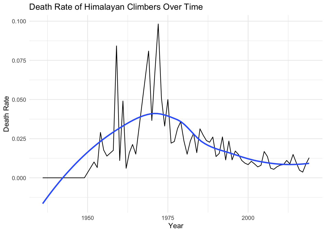
Death Rate of Himalayan Climbers Over Time: Shows how the death rate of Himalayan climbers has changed over the years.

/* Compute annual death rates by treating TRUE deaths as 1 and
   FALSE deaths as 0. The average therefore represents the
   proportion of climbers who died in a given year. We exclude
   years with fewer than 50 climbers to reduce noise from very
   small sample sizes. */

SELECT 
  e.year,
  AVG(CASE WHEN m.died = TRUE THEN 1 ELSE 0 END) AS death_rate,
  COUNT(*) AS total_climbers
FROM members m
JOIN expeditions e
  ON m.expedition_id = e.expedition_id
WHERE e.year IS NOT NULL
GROUP BY e.year
HAVING COUNT(*) > 50
ORDER BY e.year;

Displaying records 1 - 10

year	death_rate	total_climbers
1936	0.0000000	55
1949	0.0000000	61
1952	0.0101010	99
1953	0.0065789	152
1954	0.0289855	207
1955	0.0177515	169
1956	0.0138889	72
1958	0.0175439	57
1959	0.0842105	95
1960	0.0110497	181

# Execute the SQL query and store the results in an R data frame.
# This allows us to move from database analysis to visualization
# and further processing in R.

death_trend_data <- dbGetQuery(con_exp, "
SELECT 
  e.year,
  AVG(CASE WHEN m.died = TRUE THEN 1 ELSE 0 END) AS death_rate,
  COUNT(*) AS total_climbers
FROM members m
JOIN expeditions e
  ON m.expedition_id = e.expedition_id
WHERE e.year IS NOT NULL
GROUP BY e.year
HAVING COUNT(*) > 50
ORDER BY e.year
")

# Visualize how annual death rates have changed over time.
# The smooth trend line helps identify long-term patterns
# that may not be obvious from year-to-year variation.

ggplot(death_trend_data, aes(x = year, y = death_rate)) +
  geom_line() +
  geom_smooth(se = FALSE) +
  labs(
    title = "Death Rate of Himalayan Climbers Over Time",
    x = "Year",
    y = "Death Rate"
  ) +
  theme_minimal()

`geom_smooth()` using method = 'loess' and formula = 'y ~ x'

By plotting the proportion of climbers who died each year, we can see that the death rate has steadily declined since 1970, which makes sense as there has been upgrades to technology as well as more guides present on these expeditions. The data increases steadily at the start which makes sense given the smaller number of climbers in the beginning years as well as the lack of knowledge of the climb.

Continuation of Hired Staff Impact Analysis

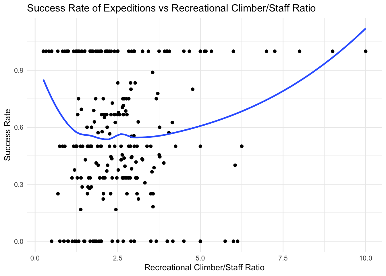
My interest here is to see if there is any positive correlation between these two. I expect that there will be some, but not extremely strong, as what really matters is the difficulty of the peak, the experience of the people, etc. But presumably more professional staff members should result in more success.

/*Query to get both the success rate and the member-staff ratio for all peaks 
without 100% or 0% success rate*/

 SELECT
    p.peak_name,
    SUM(CASE WHEN e.termination_reason LIKE '%Success%' THEN 1 ELSE 0 END) * 1.0 /
    COUNT(*) AS success_rate,
    AVG(e.members * 1.0 / e.hired_staff) AS member_staff_ratio
  FROM expeditions e
  JOIN peaks p
    ON e.peak_id = p.peak_id
  WHERE (e.members != 0 AND e.hired_staff != 0)
  GROUP BY p.peak_name

Displaying records 1 - 10

peak_name	success_rate	member_staff_ratio
Churen Himal East	0.3333333	2.877778
Manaslu	0.5765766	2.027507
Gangapurna	0.2500000	2.778472
Manaslu North	0.5000000	3.385417
Dhaulagiri II	0.4000000	1.910290
Dhaulagiri V	0.6666667	1.289855
Ngojumba Kang II	1.0000000	3.916667
Churen Himal Central	0.6666667	2.014286
Dhaulagiri VI	0.6000000	1.708333
Annapurna I East	0.7500000	2.656250

# Execute the SQL query and store the results in an R data frame.
# This allows us to move from database analysis to visualization
# and further processing in R.

success_rate_member_ratio_data <- dbGetQuery(con_exp, "
SELECT
    p.peak_name,
    SUM(CASE WHEN e.termination_reason LIKE '%Success%' THEN 1 ELSE 0 END) * 1.0 /
    COUNT(*) AS success_rate,
    AVG(e.members * 1.0 / e.hired_staff) AS member_staff_ratio
  FROM expeditions e
  JOIN peaks p
    ON e.peak_id = p.peak_id
  WHERE (e.members != 0 AND e.hired_staff != 0)
  GROUP BY p.peak_name")

# Visualize the relationship between staff support and
# expedition success. If peaks with lower climber-to-staff
# ratios tend to have higher success rates, we would expect
# to see a positive trend in the data.

ggplot(success_rate_member_ratio_data, aes(x = member_staff_ratio, y = success_rate)) +
  geom_point() +
  geom_smooth(se = FALSE)+
labs(
    title = "Success Rate of Expeditions vs Recreational Climber/Staff Ratio",
    x = "Recreational Climber/Staff Ratio",
    y = "Success Rate"
  ) +
  theme_minimal()

`geom_smooth()` using method = 'loess' and formula = 'y ~ x'

# Transfer the filtered SQL results into R for visualization.
# Peaks with success rates of exactly 0% or 100% are excluded
# so the analysis can focus on peaks with more variation in outcomes.

success_rate_member_ratio_data_filtered <- dbGetQuery(con_exp, "
 SELECT * FROM
 (SELECT
    p.peak_name,
    SUM(CASE WHEN e.termination_reason LIKE '%Success%' THEN 1 ELSE 0 END) * 1.0 /
    COUNT(*) AS success_rate,
    AVG(e.members * 1.0 / e.hired_staff) AS member_staff_ratio
  FROM expeditions e
  JOIN peaks p
    ON e.peak_id = p.peak_id
  WHERE (e.members != 0 AND e.hired_staff != 0)
  GROUP BY p.peak_name
 ) t
WHERE success_rate NOT IN (0, 1)
 ")

# Visualize the relationship between climber-to-staff ratio and
# success rate after removing peaks with 0% and 100% success rates.
# This helps reveal trends that may be obscured by extreme values.

ggplot(success_rate_member_ratio_data_filtered, aes(x = member_staff_ratio, y = success_rate)) +
  geom_point() +
  geom_smooth(se = FALSE)+
labs(
    title = "Success Rate of Expeditions vs Recreational Climber/Staff Ratio",
    x = "Recreational Climber/Staff Ratio",
    y = "Success Rate"
  ) +
  theme_minimal()

`geom_smooth()` using method = 'loess' and formula = 'y ~ x'

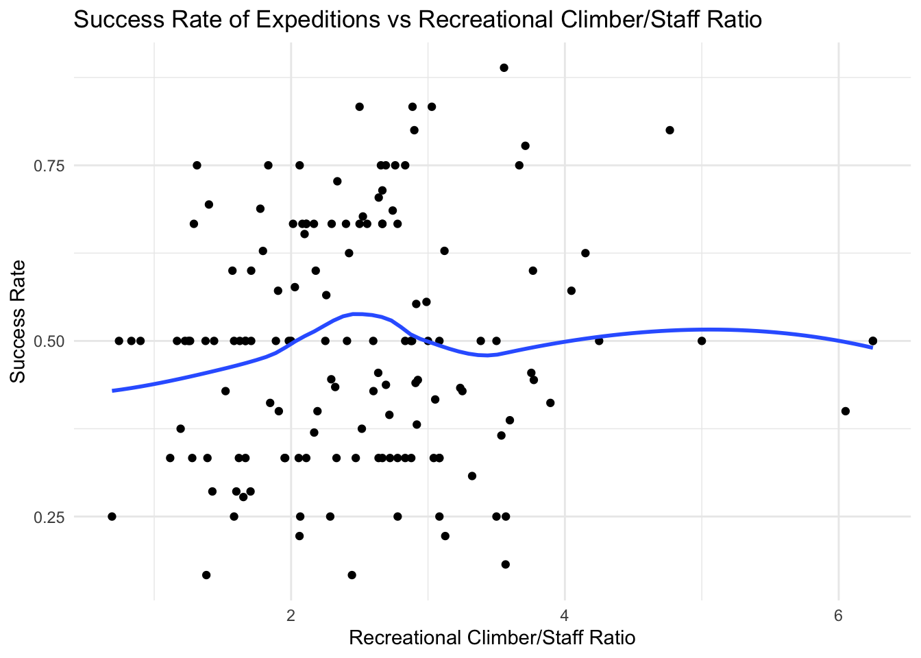
Unfiltered version seems to suggest there may be a small correlation. We do see more 100% success rates with higher ratios. However when we glance at the filtered version, it seems like there is less of one (though there may be something small). But overall I imagine other factors like experience, and peak difficulty matter the most.

—————————————————————————

# terminate the SQL connection

DBI::dbDisconnect(con_exp, shutdown = TRUE)

—————————————————————————